Numpy/SciPy¶

^{_{The stuff below is inspired from https://www.youtube.com/watch?v=8JfDAm9y_7s and https://github.com/gertingold/euroscipy-numpy-tutorial}}

	NumPy Base N-dimensional array package		Matplotlib Comprehensive 2D Plotting
	SciPy library Fundamental library for scientific computing		Pandas Data structures & analysis

^{_{https://www.scipy.org/}}

What is Numpy¶

Core library for scientific computing in Python
- It is nearly impossible to find a scientific package in Python that does not depend on numpy
Defines a multidimensional array object and the tools to work on them
- Linear algebra, DFT, random numbers, …
Has a good documentation
- https://docs.scipy.org/doc/numpy/

^{_{https://www.oreilly.com/library/view/elegant-scipy/9781491922927/ch01.html}}

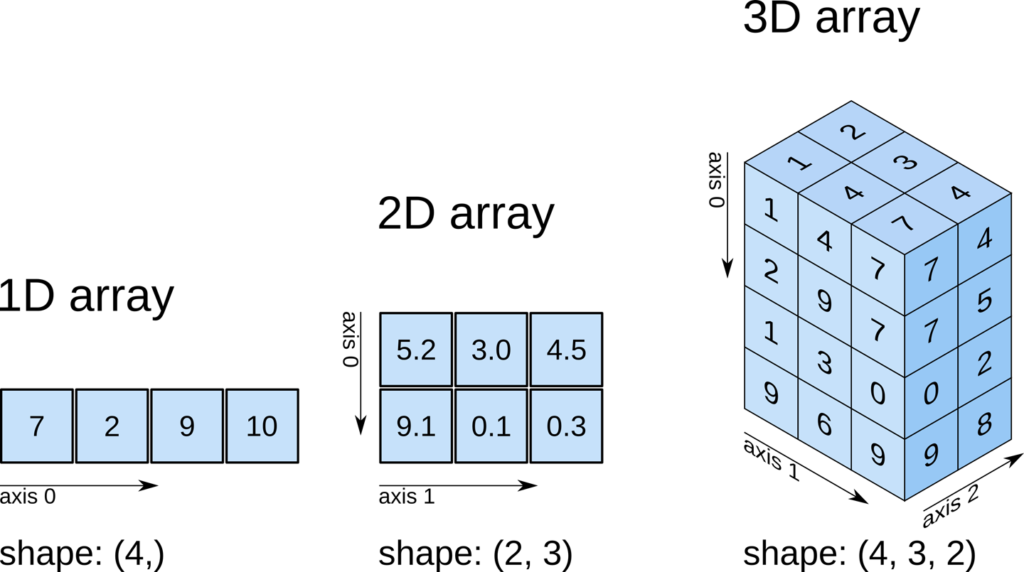
Example: Import numpy and create a 3-dimensional array with the shape [4, 3, 2]

>>> import numpy as np
>>> a = np.zeros(shape=[4, 3, 2])

Datatypes (dtype)¶

Integers: np.int8, np.int16, np.int32, np.int64, np.uint8, …
Float: np.float16, np.float32, np.float64, …
Complex: np.complex64 (single precision), np.complex128 (double precision), …
Boolean: np.bool8
default type: np.float64

Python has buildin support for complex types:

>>> 1 + 1j
(1+1j)

Note: Numpy is not save against overflows (while python is):

>>> a = np.array([200], dtype=uint8)
>>> a
array([200], dtype=uint8)
>>> a + a  # overflow
array([144], dtype=uint8)
>>> a + 200  # overflow
array([144], dtype=uint8)
>>> a + 300  # no overflow, because 300 is first converted to uint16
array([500], dtype=uint16)

Numpy vs python list¶

Less memory
- Numpy has a dtype (datatype) for the elements (Stores content as bytestream with a header that describes the content)
- Each list element can have a different type
Faster
- Numpy functions (np.sum, np.linalg.inv, np.fft.fft) are implemented in C/C++ (Blas, LAPACK, MKL, …)
- Python list has always the interpreter overhead
Easier to use for numeric problems
- Numpy supports matrix operations (np.matmul, np.einsum)

Array creation¶

Numerical ranges: np.arange, np.linspace, np.logspace, …
Homogeneous data: np.zeros, np.ones, …
Diagonal elements: np.diag, np.eye, …
Random numbers: np.random.rand, np.random.randint, …
From list: np.array

Numpy has an append()-method like python lists. Avoid it. Use a python list with append and convert it with np.array

Numpy array properties¶

>>> a.shape  # the shape of the array
(4, 3, 2)
>>> a.ndim  # the number of dimensions of the array
3
>>> a.dtype  # the dtype of the array
np.float64
>>> a.size  # the number of elements
24
>>> len(a)  # Note: len returns the length of the fist dimension to be compatible with python lists
4
>>> a.strides  # Memory step that corresponds to an index increase
(48, 16, 8)

Strides are one reason for the efficiency of numpy. Usually the user does not care about the strides.

Transpose¶

A transpose in numpy means array transpose and not matrix transpose

>>> a.shape
(4, 3, 2)
>>> b = a.T  # array transpose
>>> b.shape
(2, 3, 4)
>>> a.transpose(0, 2, 1).shape
(4, 2, 3)
>>> np.swapaxes(a, -1, -2).shape  # matrix transpose
(4, 2, 3)

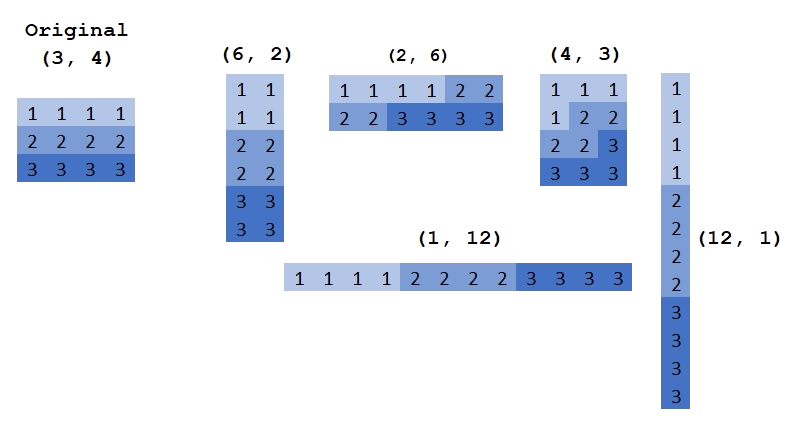
Reshape¶

You can change the shape of an array with reshape. The numbers after reshape are the same, only the arrangement changes.

>>> a = np.array([[1, 1, 1, 1], [2, 2, 2, 2], [3, 3, 3, 3]])
>>> a
array([[1, 1, 1, 1],
       [2, 2, 2, 2],
       [3, 3, 3, 3]])
>>> b = a.reshape(2, 6)  # same as np.reshape(a, [2, 6])
>>> b
array([[1, 1, 1, 1, 2, 2],
       [2, 2, 3, 3, 3, 3]])

^{_{http://backtobazics.com/wp-content/uploads/2018/08/numpy-reshape-examples.jpg}}

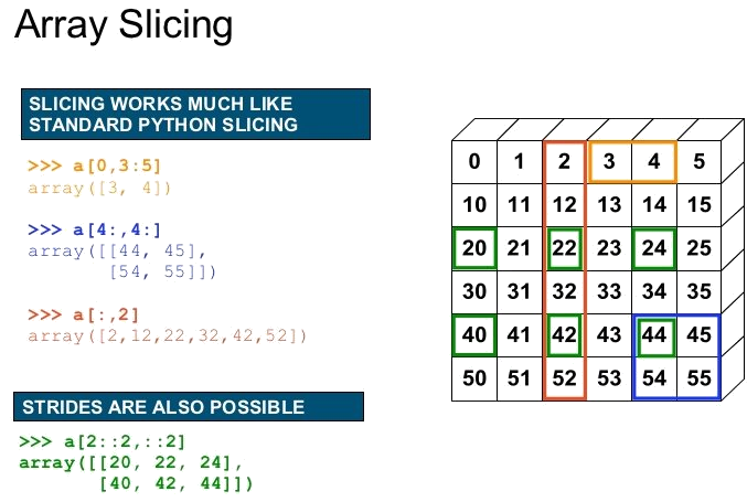
Getitem: Slicing and indexing¶

In python the index starts with 0 like in C/C++ and not with 1 as in MATLAB. The syntax is: [start:stop:step]. Step describes the spacing between two values and is optional [start:stop] with a default value of 1. Negative values are supported (e.g [::-1] reverses the order). A value for start [:stop] and stop [start:] is also optional (defaults: start=0 and stop=N where N is the length of the dimension). Examples (1 dimensional):

^{_{https://github.com/gertingold/euroscipy-numpy-tutorial/tree/master/images}}

Note: The last value is not included in slicing (e.g. [:-1] mean drop the last element)

Negative indices for start and stop are also supported:

^{_{https://github.com/gertingold/euroscipy-numpy-tutorial/tree/master/images}}

Some 1 dimensinal code examples:

>>> a = np.arange(5)
>>> a
array([0, 1, 2, 3, 4])
>>> a[0]  # Index with a scalar
0
>>> a[:]  # slice with a column, here all values
array([0, 1, 2, 3, 4])
>>> a[1:]  # values from index 1 to the end
array([1, 2, 3, 4])
>>> a[:-1]  # values from begin to the last, but exclude the last. Note negative indices are allowed
array([0, 1, 2, 3])
>>> a[::2]  # Take each second value
array([0, 2, 4])
>>> start, end, step = 1, 4, 2
>>> a[start:end:step]  # Use all of them (start, stop, step)
array([1, 3])
>>> a[...]  # The "ellipsis" in getitem, see for eplanation below
array([0, 1, 2, 3, 4])

Ellipsis: The ellipsis (...) is a special argument to getitem ([ ]). It is used to handle an unknown number of dimensions. It means fill the getitem with so many colons (:) that on all dimensions an slicing/indexing is used.

Higher dimensional slicing with ellipsis:

>>> a = np.arange(4*3*2).reshape(4, 3, 2)
>>> a[..., 0]  # equal to a[:, :, 0]
array([[ 0,  2,  4],
       [ 6,  8, 10],
       [12, 14, 16],
       [18, 20, 22]])
>>> a[0, ..., 1]  # equal to a[0, :, 1]
array([1, 3, 5])
>>> a = np.arange(4*3).reshape(4, 3)
>>> a
array([[ 0,  1,  2],
       [ 3,  4,  5],
       [ 6,  7,  8],
       [ 9, 10, 11]])
>>> a[..., 0]  # equal to a[:, 0]
array([0, 3, 6, 9])
>>> a[0, ..., 1]  # equal to a[0, 1]
array(1)

and a visualisation ^{_{https://image.slidesharecdn.com/numpytalksiam-110305000848-phpapp01/95/numpy-talk-at-siam-14-728.jpg?cb=1299283822}}

Two advanced indexing examples. One with a boolean mask and the other one with an array of integers (% is modulo in Python):

^{_{https://github.com/gertingold/euroscipy-numpy-tutorial/tree/master/images}}

Function¶

The np.ndarray in numpy has many methods to manipulate itself (a.max(), a.sum(), a.reshape(), …). These have always a counterpart in the numpy namespace (np.max(a), np.sum(a), np.reshape(a), …). These functions will also work where a is compatible with numpy, i.e. np.max(a) is equal to np.max(np.array(a)).

By default most numpy reduction functions perform the operation on the full array. For example np.sum(a) returns the sum of all elements of a, independent of the numer of dimensions of a. To perform a operation on a specific dimension these functions have an axis argument:

>>> a = np.arange(4*3*2).reshape(4, 3, 2)
>>> a
array([[[ 0,  1],
        [ 2,  3],
        [ 4,  5]],

       [[ 6,  7],
        [ 8,  9],
        [10, 11]],

       [[12, 13],
        [14, 15],
        [16, 17]],

       [[18, 19],
        [20, 21],
        [22, 23]]])
>>> np.sum(a)
276
>>> np.sum(a, axis=-1)
array([[ 1,  5,  9],
       [13, 17, 21],
       [25, 29, 33],
       [37, 41, 45]])
>>> np.sum(a, axis=(-2, -1))
array([ 15,  51,  87, 123])

Some example operations:

>>> a = np.arange(5)
>>> a ** 2  # square, in python ** is the pow operator
array([ 0,  1,  4,  9, 16])
>>> a + a
array([0, 2, 4, 6, 8])
>>> a + 2
array([2, 3, 4, 5, 6])
>>> np.sqrt(a)
array([0.        , 1.        , 1.41421356, 1.73205081, 2.        ])

and there are many more functions, for example (all of them are in the numpy namespace np):

Trigonometric functions
- sin, cos, tan, arcsin, arccos, arctan, hypot, arctan2, degrees, radians, unwrap, deg2rad, rad2deg
Other special functions
- i0, sinc
Hyperbolic functions
- sinh, cosh, tanh, arcsinh, arccosh, arctanh
Rounding
- around, round_, rint, fix, floor, ceil, trunc
Floating point routines
- signbit, copysign, frexp, ldexp
Arithmetic operations
- add, reciprocal, negative, multiply, divide, power, subtract, true_divide, floor_divide, fmod, mod, modf, remainder
Sums, products, differences
- prod, sum, nansum, cumprod, cumsum, diff, ediff1d, gradient, cross, trapz
Handling complex numbers
- angle, real, imag, conj
Exponents and logarithms
- exp, expm1, exp2, log, log10, log2, log1p, logaddexp, logaddexp2
Miscellaneous
- convolve, clip, sqrt, square, absolute, fabs, sign, maximum, minimum, fmax, fmin, nan_to_num, real_if_close, interp
Matrix and vector products
- dot, vdot, inner, outer, matmul, tensordot, einsum, linalg.matrix_power, kron
Decompositions
- linalg.cholesky, linalg.qr, linalg.svd
Matrix eigenvalues
- linalg.eig, linalg.eigh, linalg.eigvals, linalg.eigvalsh
Norms and other numbers
- linalg.norm, linalg.cond, linalg.det, linalg.matrix_rank, linalg.slogdet, trace
Solving equations and inverting matrices
- linalg.solve, linalg.tensorsolve, linalg.lstsq, linalg.inv, linalg.pinv, linalg.tensorinv
Order statistics
- amin, amax, nanmin, nanmax, ptp, percentile, nanpercentile
Averages and variances
- median, average, mean, std, var, nanmedian, nanmean, nanstd, nanvar
Correlating
- corrcoef, correlate, cov
Histograms
- histogram, histogram2d, histogramdd, bincount, digitize
Sorting
- sort, lexsort, argsort, msort, sort_complex, partition, argpartition
Searching
- argmax, nanargmax, argmin, nanargmin, argwhere, nonzero, flatnonzero, where, searchsorted, extract
Counting
- count_nonzero
…

^{_{https://github.com/gertingold/euroscipy-numpy-tutorial/}}

One often used operation is the matrix multiplication. For the matrix multiplication there are 3 ways to execute it:

np.matmul(A, b) is the recommented one (or the @ operator)
A @ b alternative syntax for np.matmul
np.dot(A, b) similar to np.matmul but has difference broadcasting behaviours.

Note: A * b is the elementwise multiplication

Broadcasting¶

By default the python operators (+, -, *, /, **) operate elementwise (except matrix multiplication @). To work elementwise it is important that the shapes match. At this position broadcasting is important. It mean, when the shapes do not match, numpy try to match them with broadcasting.

Broadcasting rules:

The arrays all have exactly the same shape.
The arrays all have the same number of dimensions and the length of each dimension is either a common length or 1.
The arrays that have too few dimensions can have their shapes prepended with a dimension of length 1 to satisfy property 2.

^{_{https://github.com/gertingold/euroscipy-numpy-tutorial/}}

^{_{https://github.com/gertingold/euroscipy-numpy-tutorial/tree/master/images}}

Getitem: Insert singleton dimension¶

>>> a = np.array([1, 2, 3])
>>> b = np.array([5, 11])
>>> a[None, :].shape
(1, 3)
>>> b[:, np.newaxis].shape
(2, 1)
>>> a[None, :] + b[:, np.newaxis]
array([[ 6,  7,  8],
       [12, 13, 14]])

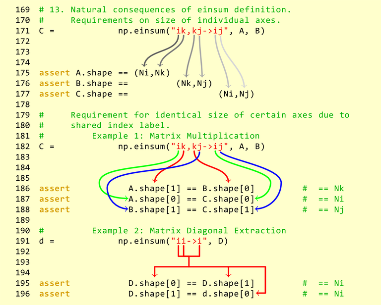
Einsum¶

https://en.wikipedia.org/wiki/Einstein_notation

^{_{https://obilaniu6266h16.wordpress.com/2016/02/04/einstein-summation-in-numpy/}}

Further information¶

Numpy is a very well documented library
- do an online search for a function and you find a description with some toy exampls.
When this introduction was not enough, there are many further online tutorials
On stackoverflow are many examples for specific problems